One of the skills that Abaqus application engineers need to know is first to understand the commands of Abaqus Input files and then to be able to modify and edit them. In this Abaqus blog, we try to have a useful general description of the structure of the input file, as well as a useful tool to download Input documentation files without the need to install it.
Built-in Tool for Abaqus Input Files (*.inp)
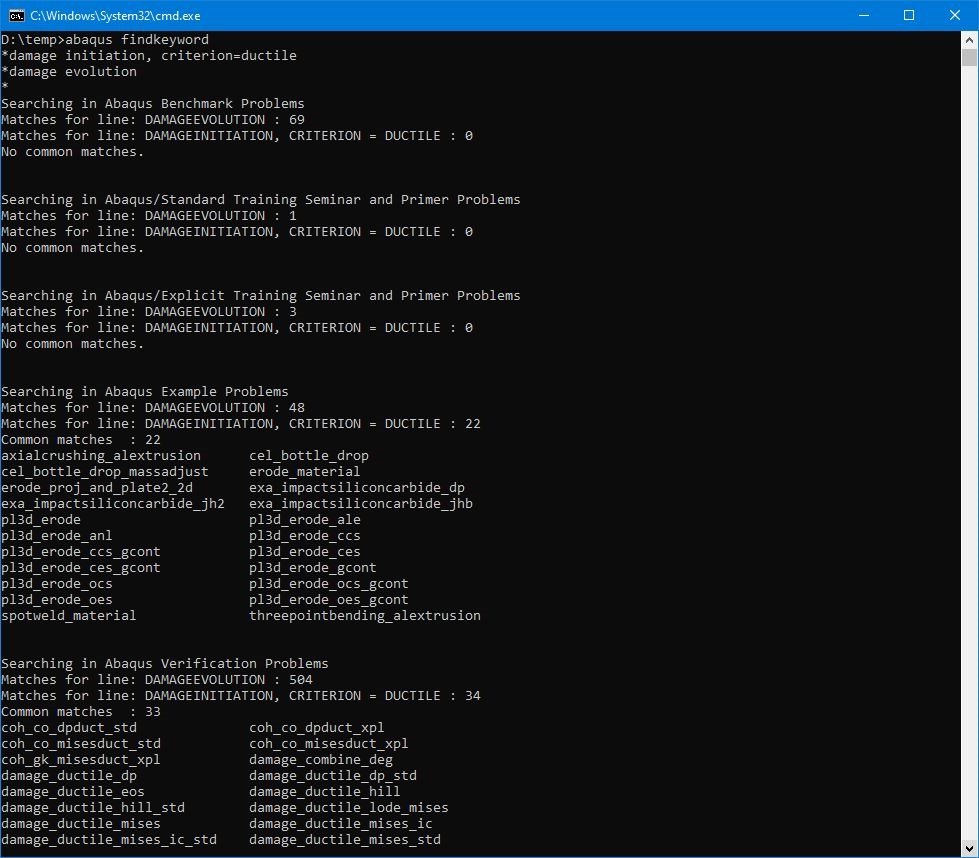
A lot of Abaqus users don’t know that still, there is an Abaqus built-in tool to easily search through all examples, benchmarks, verification, and training input files for specific keywords and parameters. You don’t need to have the Abaqus documentation installed locally, since the files and tools come with the core Abaqus installation.
Run this command to search in those input files:
>abaqus findkeywordNow you can enter the keywords and parameters you are looking for.
It will generate a list with all files that match your query.
Afterward, you can use the fetch command to extract the file you want to further inspect.
>abaqus fetch job=filenameIt will copy the file into your current work directory.
What is the Abaqus Input Files (*.inp)?
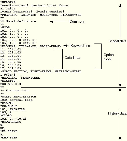
The input file is the interface between the Abaqus/CAE preprocessor and the analysis obtained from the Abaqus solver and written with ASCII code including a complete description of the numerical model. The input file is a text file that contains information about the model and the history of the model. These files have almost the same structure.
This file includes keyword lines and data lines. The input file usually starts with *HEADING. Of course, it is not necessary and its absence is not a problem. After this option is model data and then history data.
If a preprocessor such as Abaqus/CAE is used, it can be modified with it. In fact, for small analysis, it is very easy to type in the input file.
Model Data
Model data includes information related to the definition of nodes and elements, type of material, initial conditions, etc.
A subset of model data is described below.
Parts and an assembly: Model geometry and things related to parts and how to connect.
Initial conditions: non-zero initial conditions, such as initial stress, temperature, or velocity that are specified.
Boundary conditions: Zero-valued boundary conditions (including symmetry conditions) can be imposed on individual solution variables such as displacements or rotations.
Kinematic constraints: Equations involving several of the fundamental solution variables in the model or multi-point constraints can be defined.
Interactions: Contact and other interactions between parts can be defined.
Amplitude definitions: Amplitude curves can be defined for later use in specifying time-dependent loading or boundary conditions.
Output control: You can control the model definition output to the data file.
Environment properties: Environment properties, such as the attributes of a fluid surrounding the model, may have to be defined.
Analysis continuation: It is possible to write restart data or to use the results from a previous analysis and continue the analysis with a new model or history data.
History data
This section starts with *STEP and ends with *END STEP.
Keyword lines
In the inp file, the blocks containing information about the model’s parts are written. Each block starts with a key line, which is usually followed by a line or lines that these lines cannot be more than 256 characters. The keywords usually start with an Asterisk (*) at the beginning. Like *NODE, a keyword for specifying node coordinates, and* ELEMENT Keywords for element connection specifications. Keywords are often accompanied by parameters that come after them and are required. The TYPE parameter comes after *ELEMENT and specifies the element type.
for example:
*ELEMENT, TYPE=T2D2
which shows that we have defined the connection of elements T2D2. two-dimensional truss element with two nodes, many parameters are optional and are defined for a specific part.
for example:
*NODE, NSET=PART1
which shows that all the nodes defined in this block are all from the same SET that it is called PART1.
Data lines
It is usually followed by keyword lines and data lines. Very simple in the form of a list of parameters that come after the keyword line. This information includes coordinates, Nodes, connection of elements, table of material properties, etc.
*NODE
101, 0., 0., 0.
102, 1., 0., 0.
103, 2., 0., 0.
104, 0.5, 0.866, 0.
The first part of each line is the number of the node and the rest is the coordinates of that node. (x1, x2, x3). this information can contain integer, float, & alphabet letters. An integer can be entered in several ways. As:
4.0 4. 4
4.0E+0 .4E+1 40.E−1
Any line in the input file that begins with two stars (**) is an explanation, interpretation, and comment. it does not have a computational or command role.
How to Open Abaqus INP file in LS-Dyna?
Another question that is very common is how to run the Abaqus input file in LS-Dyna. You can use the following Abaqus tutorial for this purpose.
How to Export Abaqus Input file?
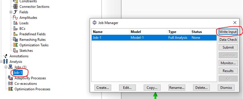
Exporting the Abaqus input file is very simple. After building the model in the Abaqus CAE graphical interface, in the job module, create a job and then hit Write Input, now a file with the extension *.inp will be generated in your directory.
We hope this article was useful for you. Do not miss this Built-in Material Models in Abaqus article.

