The Ultimate Guide to the XFEM Method in Abaqus for Crack Propagation

Simulating how materials fail and how cracks grow is one of the most complex challenges in modern finite element analysis (FEA). Traditional numerical methods often struggle with moving boundaries, requiring tedious and computationally expensive re-meshing strategies.

This is where the XFEM Method in Abaqus (eXtended Finite Element Method) revolutionizes fracture mechanics. By allowing local enrichment functions to capture the singularity at the crack tip, XFEM enables simulation engineers to model stationary and moving cracks independently of the finite element mesh.

What is the eXtended Finite Element Method (XFEM)?

The Abaqus XFEM technique extends the capabilities of standard finite element analysis. Introduced to represent discontinuities (such as cracks) within elements, it eliminates the need for explicit meshing of crack surfaces.

In Abaqus, XFEM is implemented by enriching the standard finite element approximation with additional enrichment functions. These functions represent the displacement field near the crack tip, providing highly accurate stress solutions. This means you can study crack growth along an arbitrary, solution-dependent path without ever needing to re-mesh your model.

Industrial Applications of Abaqus XFEM

XFEM is not just a theoretical tool; it solves real-world industrial problems. Engineers use Abaqus XFEM crack propagation techniques to evaluate critical failures, including:

• Hydrogen-induced cracking (HIC) in oil and gas pipelines.
• Stress corrosion cracking in marine and offshore structures.
• Fatigue and fracture mechanics in aerospace composites.
• Predicting failure in 2D and 3D complex metal geometries.
• Fitness-for-Service Assessment (FFS)
• Failure Analysis

If you want to know more about Abaqus projects, check out Abaqus projects

Step-by-Step Abaqus XFEM Tutorial: Plate with a Hole

In this tutorial, we will use the standard Abaqus solver to predict both crack initiation and propagation due to stress concentration in a 2D plate with a hole subjected to tension.

Part and Mesh Module Strategies

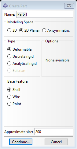
Start by creating a 2D deformable part (a rectangle with a circular hole on one edge). Partitioning the space around the hole is highly recommended to control the mesh density. In the Mesh Module, apply a small, refined mesh size in the region with high stress concentration using standard linear plane strain elements (CPE4R). Mesh independence is a key benefit of the XFEM method in Abaqus, but a refined mesh near the crack path improves accuracy.

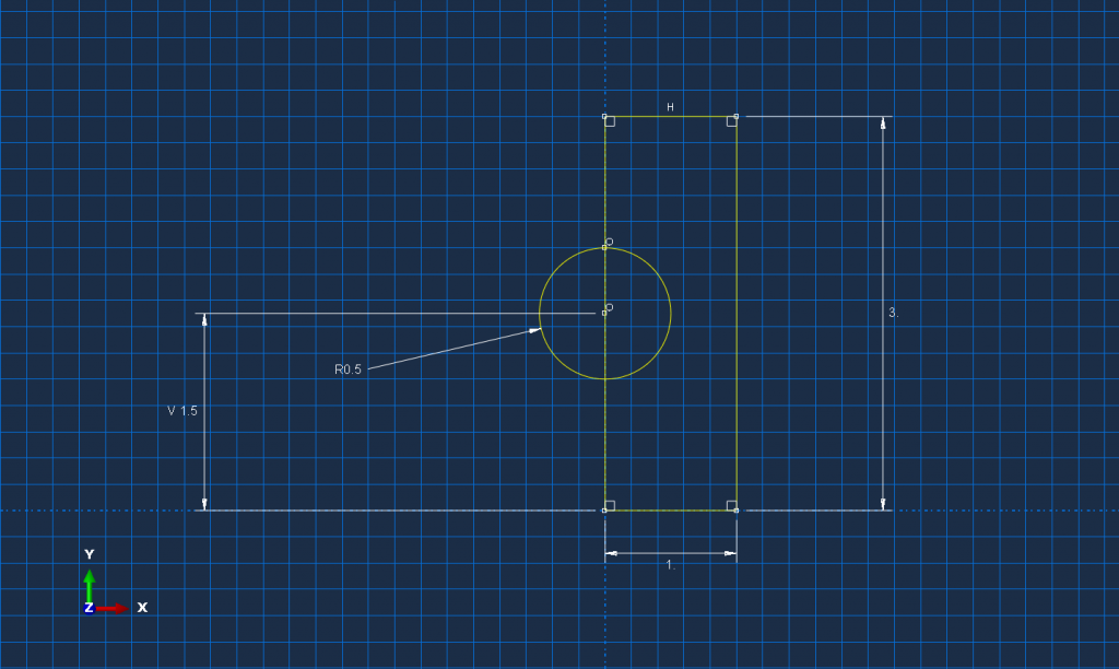
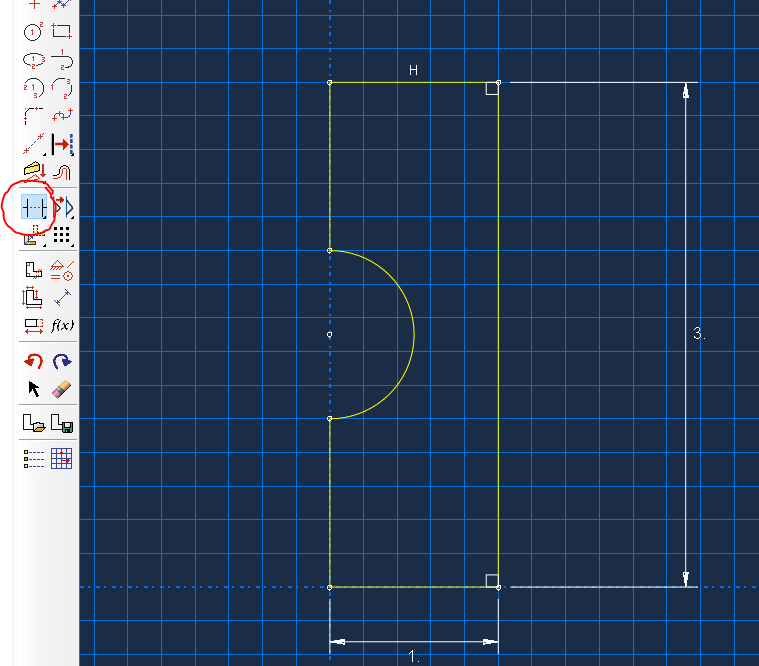
Next, create a circle in the middle of the left side with a radius of 0.5. After that, it needs to trim redundant curves.

Property Module: Defining Damage Criteria

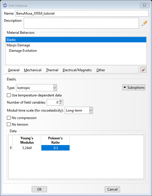
Create a material with linear elastic behavior. Next, we must define the traction-separation behavior using the Maximum Principal Stress criterion. If the maximum principal stress reaches a critical positive value, the crack initiates. You must also define the Damage Evolution rule based on energy and linear softening. For mixed-mode fracture, using the BK (Benzeggagh-Kenan) formulation allows you to calculate the effective energy release rate (G_1, G_2, G_3).

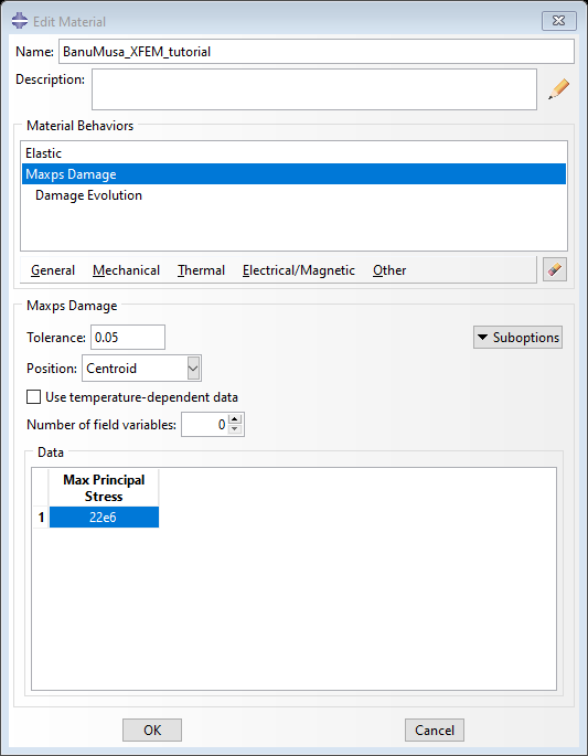
As you can see in this criterion, if the maximum principal stress is positive and more than a critical value, the crack initiates and propagates. If the value of this function is between 1 and 1 + tolerance, the crack initiation will be considered in the next increments. But if the value is more than one plus tolerance, this increment will be solved one more time by cutback.

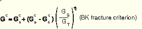
Then define the damage evolution rule based on energy and linear softening. Also, use the BK (Benzeggagh-Kenan) formulation to calculate the effective energy release rate from the energy illustrated in various models.

as it is shown in this formula, it needs to enter the power.

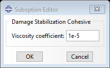
then enter critical values of G1, G2, and G3. Also, use a stabilization option to simplify the convergence of the standard solver.

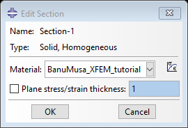
Next, create a section and assign it to the part.

(Pro Tip: Calibrating damage properties for fracture mechanics is notoriously difficult. Instead of manual trial and error, you can instantly import validated fracture material data using our Abaqus Material Library (MatLib).

Assembly Module

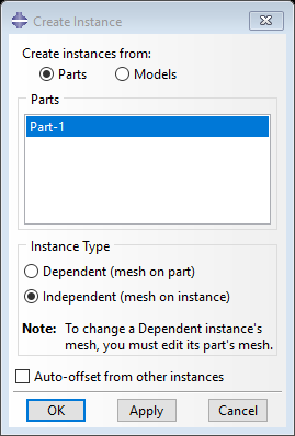
Then insert the part in the assembly module.

Step and Interaction Modules

Since crack propagation introduces severe non-linearities, setting up the Step module correctly is vital.

• Create a Static, General step.
• Reduce the initial increment size and increase the maximum number of increments to help the solver converge.
• In the Field Output requests, ensure you check the boxes for PHILSM (Signed distance function to describe the crack surface) and STATUSXFEM (State of the enriched elements).

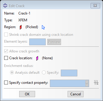
In the Interaction module, create an XFEM Crack and select your target domain. While you can define an initial crack here, the software will automatically determine the crack path based on your damage criteria.

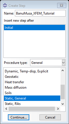
In the step module, create a static general step.

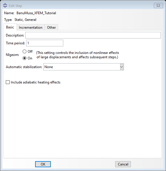
As the convergence of the problem is not easy due to the propagation of the crack. so reduce the initial minimum and maximum size of increments. also, it needs to increase the maximum number of increments.

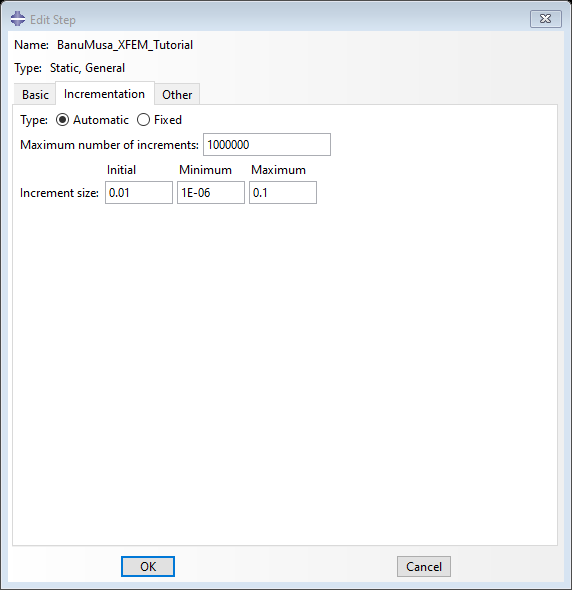
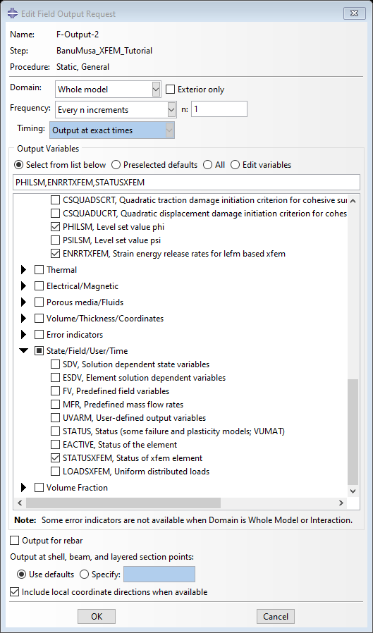
Also, request two field outputs related to the enriched elements. The first one is the sign distance function to describe the correct surface. The second one is a state of XFEM elements.

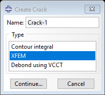
In the interaction module, we create an XFEM crack and then select the domain. Here we can also define the initial crack or specify contact properties. But it is not needed in this Abaqus XFEM example.

Load and Job Modules

Apply the appropriate boundary conditions (e.g., X-symmetry on the left side, fixed Y-displacement at the bottom, and a tensile displacement on the top edge). Submit the job and monitor the convergence. Using the stabilization options in the material definition often helps the standard solver overcome cutbacks during total element failure.

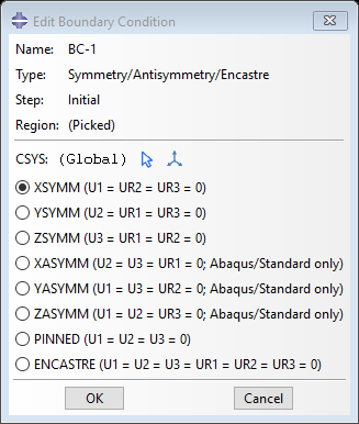
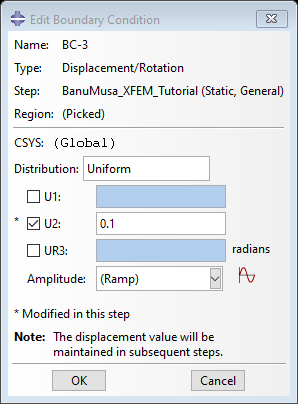
The bottom face is fixed in the y-direction, and displacement is applied to the upper edge in this direction.

Mesh Module XFEM Method in ABAQUS

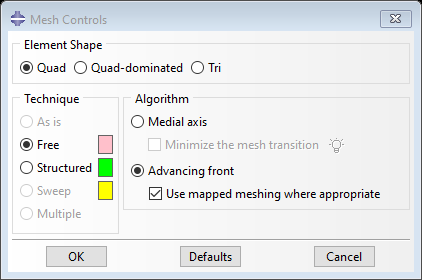
In the mesh module, first use the seed edge option. Apply a small mesh size in the region with stress concentration. We choose the quadrilateral and structured elements and then assign element types to the part.

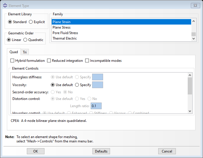
Elements are standard linear and plain strain, finally.

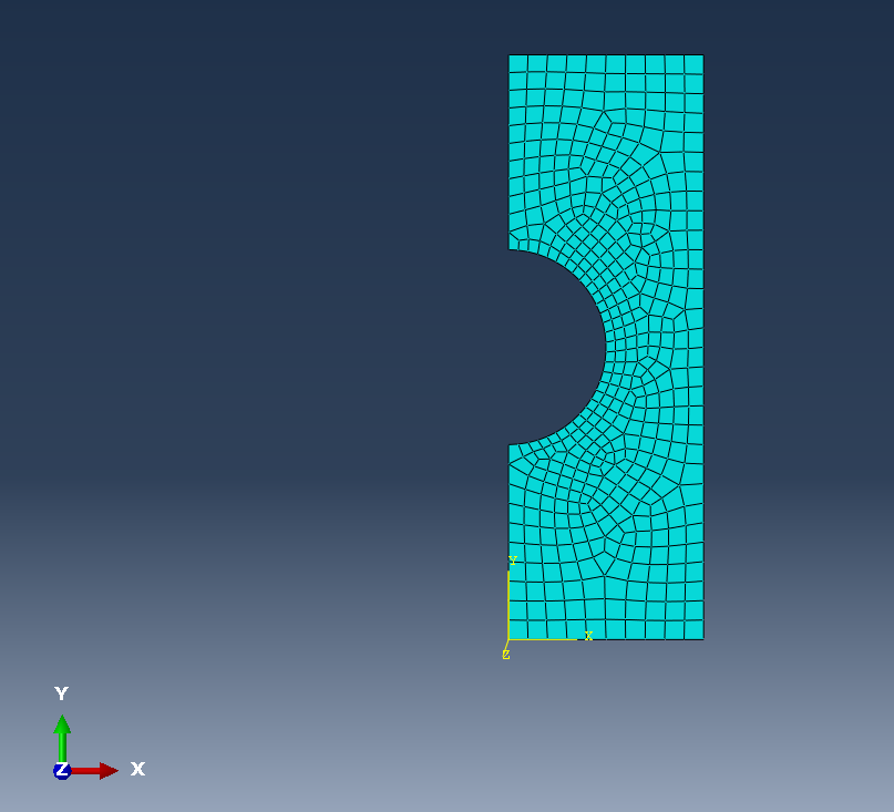
Next, generate the mesh.

Job Module XFEM Method in ABAQUS

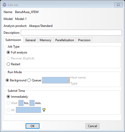
In the Job module, create the job and submit it.

Post-Processing in the Visualization Module

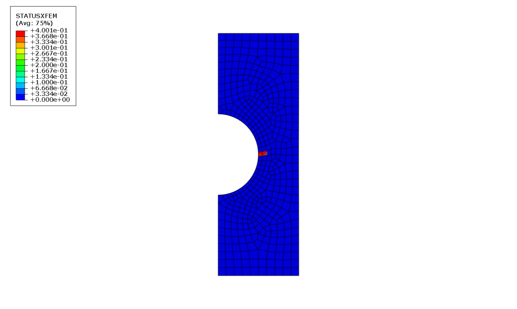
Once the job completes, load the .odb file. You can observe the crack initiation beside the hole and its subsequent propagation. Pull out the contour for PHILSM to see the distance of points from the crack surface, and view STATUSXFEM (values between 0 and 1) to identify fully fractured elements.

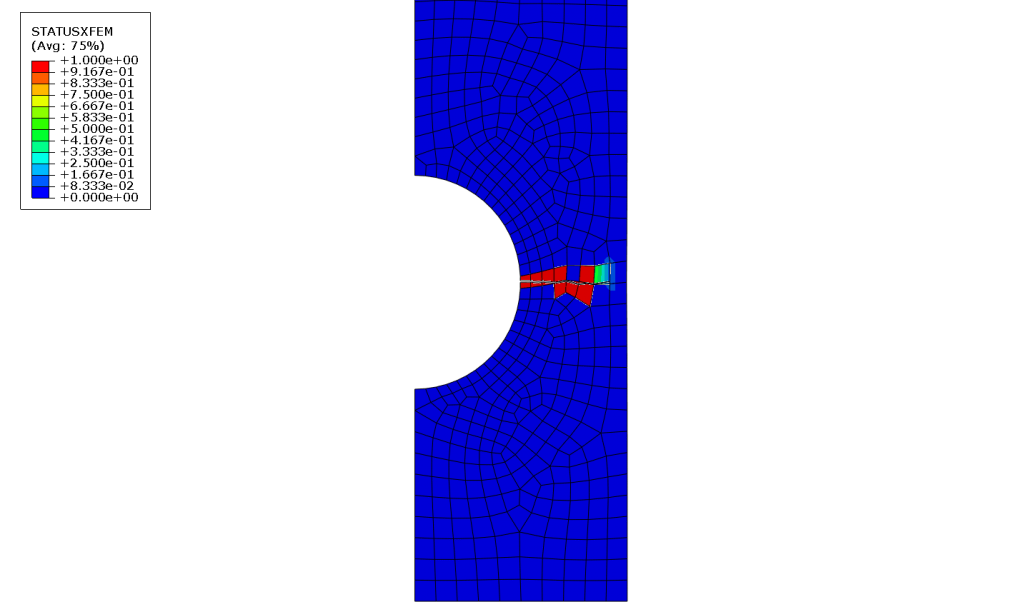
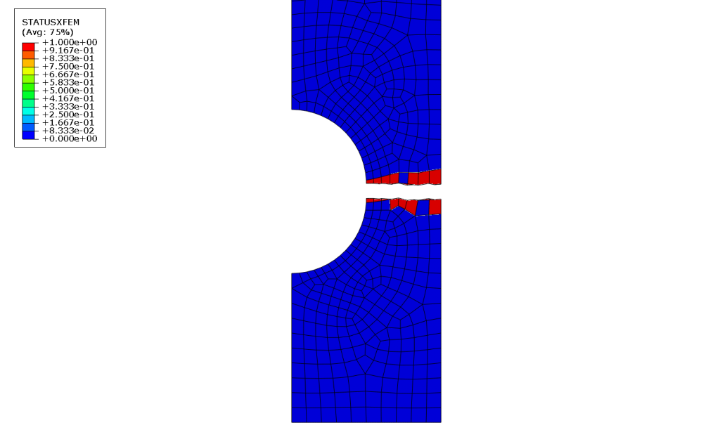
The status of an enriched element lies between 0 and 1 for correct elements.

Download the XFEM Abaqus Tutorial Files

Ready to try it yourself? You can download the complete CAE and INP files for this Abaqus XFEM crack propagation example below to see exactly how the parameters were defined.

XFEM Abaqus Tutorial Free Download

Need Expert Guidance on Fracture Mechanics?

Simulating realistic crack propagation often requires troubleshooting beyond standard tutorials. The engineering team at BanuMusa R&D offers specialized FEA and CFD consultancy, as well as dedicated Abaqus mentoring to help you overcome convergence issues and optimize your fracture models.

• Contact our Consultants: Professional FEA Consulting Services